Coin Toss & Dice Roll Probability Calculator (Exact + Simulation)

🎲 Overview – Coin Toss Probability Calculator & Dice Roll Simulator

This interactive Coin & Dice Probability Lab combines a coin toss probability calculator with a dice roll probability simulator in one browser-based tool. It is ideal for students, teachers, data-science beginners and board-game designers who want to understand how random experiments behave in practice.

The coin module lets you:

• Choose the number of coin tosses n.
• Switch between a fair coin (p(heads) = 0.5) and a biased coin with any probability of heads between 0 and 1.
• Ask questions such as exactly k heads, no heads, or at least one head.
• Compare the result with “1 in N” odds for quick intuition.

The dice module allows you to:

• Roll one up to many dice (for example 1–10 six-sided dice).
• Use a fair die (all faces are equally likely) or a custom / loaded die with your own face probabilities.
• Analyse events such as “at least one 6”, “exactly two 3s” or a sum of dice ≥ target value.
• See how frequently each total appears when you repeat the experiment many times.

For each setup the lab computes:

• A mathematically correct exact probability (0–1 and percentage).
• An intuitive “1 in N” odds description.
• A Monte Carlo simulation (thousands of virtual experiments).
• A chart comparing theoretical vs simulated results plus a short list of randomly generated example experiments.
• Export options to copy, print or save a PDF snapshot of your last calculation – perfect for homework, lesson slides or lab reports.

Together with other probability tools on SwissKnifeCalculator — such as the Ball & Urn Probability Calculator, the Deck of Cards Probability Calculator and the Advanced Random Number Generator — this lab forms a complete probability & statistics toolkit for school, university or self-study.

📚 Educational note: This coin and dice probability calculator is created for learning, teaching and intuition-building. It is not a gambling system and does not increase your chances of winning in any real-life game.

How to read your result panel

• Exact probability: the theoretical value based on probability formulas.
• Percentage: the same value shown as a percentage, e.g. 0.1172 → 11.72 %.
• “1 in N” odds: how often the event would occur on average if you repeated the whole experiment many times.
• Simulation result: how often the event actually occurred in your Monte Carlo trials: useful to check how theory and reality line up.
• Example runs: a few randomly generated sequences of tosses or rolls that match your configuration so you can see what typical outcomes look like.

📘 Formulas & Methodology – Binomial, Multinomial & Monte Carlo

Under the hood the Coin & Dice Probability Lab is powered by binomial and multinomial probability models, combined with Monte Carlo simulation to show how theory behaves in practice.

1️⃣ Coin tosses – binomial distribution

A sequence of coin tosses is a classic Bernoulli process. Let:

• n = number of tosses
• p = probability of “success” (for example heads)
• X = number of successes (heads) in n tosses

For a fair coin p = 0.5. For a biased coin you choose any p between 0 and 1. The probability of exactly k heads is given by the binomial formula:

P(X = k) = C(n, k) · p^k · (1 − p)^(n − k)

The calculator uses this expression whenever you request “exactly k heads” in the coin module.

“At least / at most” questions are handled by summing or complementing binomial probabilities, for example:

• P(X ≤ 2) = P(X = 0) + P(X = 1) + P(X = 2)
• P(X ≥ 1) = 1 − P(X = 0)

2️⃣ Dice rolls – binomial view for a target face

Many dice problems are also “success vs failure” experiments. For a fair six-sided die:

• p = 1/6 for “rolled the target face” (for example a 6)
• 1 − p = 5/6 for “anything else”

If you roll a die n times and define success as “rolled a 6”, the probability of exactly k sixes is again:

P(X = k) = C(n, k) · (1/6)^k · (5/6)^(n − k)

This is how the tool answers questions like “exactly two 3s in 6 rolls” or “at least one 6 in 4 rolls”.

3️⃣ Loaded dice – multinomial distribution

For a custom or loaded die, each face can have its own probability p1, …, p6 with p1 + … + p6 = 1. After n rolls the joint probability of seeing counts (x1, …, x6) is:

P(X1 = x1, …, X6 = x6) =
  n! / (x1! x2! … x6!) · p1^x1 · … · p6^x6

The lab uses this structure to compute expected frequencies and to generate theoretical histograms of face counts that can be compared with your simulated rolls.

4️⃣ Sums of dice – exact vs simulation

For small numbers of dice (for example 2 or 3) the tool can enumerate all outcomes exactly. With three dice there are 6^3 = 216 possible triples. For larger numbers of dice, a high-quality Monte Carlo simulation is used so calculations remain fast in your browser.

5️⃣ Monte Carlo engine & random numbers

The simulation module runs thousands of virtual experiments using JavaScript’s pseudo-random number generator. Each trial reproduces your full configuration (number of tosses, coin bias, number of dice, target event, etc.) and records whether the event occurred.

The fraction of successful trials gives the simulated probability. As you increase the number of trials, this value will typically move closer to the theoretical value — a practical illustration of the Law of Large Numbers.

🔐 These random numbers are suitable for education and general simulations, but they are not cryptographically secure and should not be used for security-sensitive applications.

🧪 Worked Examples – Coin & Dice Problems You Can Reproduce

The following examples are chosen so that they can be reproduced directly inside the Coin & Dice Probability Lab. Percentages and “1 in N” odds are rounded but match the calculator results very closely.

Example 1 – Exactly 3 heads in 10 fair tosses

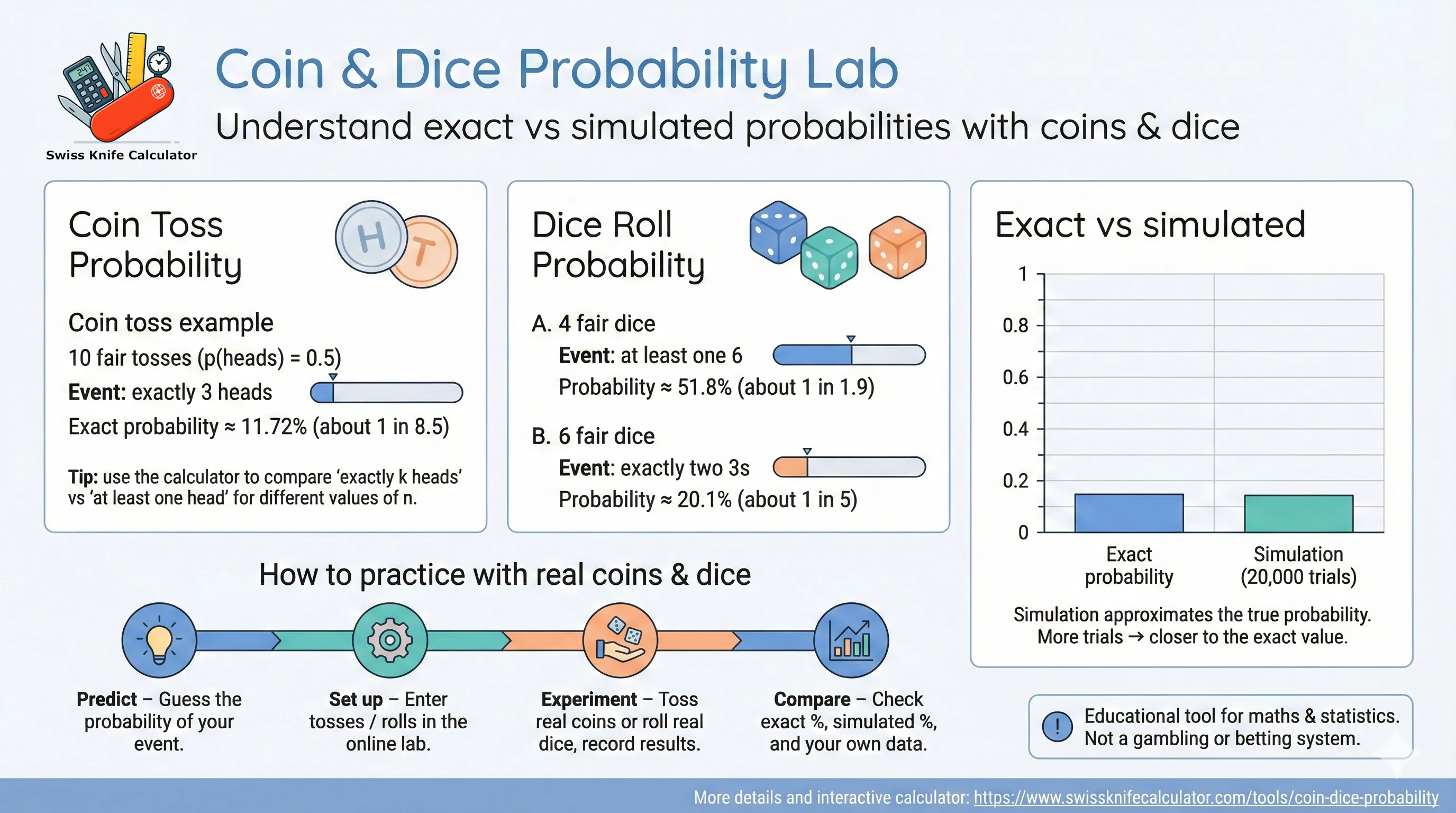
Toss a fair coin 10 times. What is the probability of exactly 3 heads?

• n = 10 tosses
• p = 0.5 (fair coin)
• k = 3 successes (heads)

P(X = 3) = C(10, 3) · 0.5^10 ≈ 0.1172

That is about 11.72 %, or roughly “1 in 8.5” ten-toss experiments. In the lab select the coin mode, set n = 10, choose “exactly k heads” and set k = 3.

Example 2 – At least one head in 5 tosses

Toss a fair coin 5 times. What is the chance of getting at least one head?

Compute the complement “no heads” and subtract from 1:

P(no heads)        = 0.5^5 = 1/32
P(at least 1 head) = 1 − 1/32 = 31/32 ≈ 0.9688

So the probability is about 96.88 % — this event is “almost certain”. In the calculator choose “at least one head” and n = 5.

Example 3 – Biased coin, 60 % chance of heads

A coin is biased so that p(heads) = 0.6. You toss it 8 times. What is the probability of getting exactly 5 heads?

• n = 8, k = 5, p = 0.6

P(X = 5) = C(8, 5) · 0.6^5 · 0.4^3 ≈ 0.2787

This is about 27.9 %, or roughly “1 in 3.6” eight-toss experiments. In the lab, set n = 8, k = 5 and move the coin-bias slider to 0.6.

Example 4 – At least one 6 in 4 rolls

Roll a fair 6-sided die 4 times. What is the probability of getting at least one 6?

P(no 6 in one roll)  = 5/6
P(no 6 in 4 rolls)   = (5/6)^4 ≈ 0.4823
P(at least one 6)    = 1 − (5/6)^4 ≈ 0.5177

So the probability is about 51.8 %, or “about 1 in 1.9” four-roll experiments. In the dice module choose 4 rolls and event “at least one target face = 6”.

Example 5 – Exactly two 3s in 6 rolls

Roll a fair die 6 times. What is the chance of seeing exactly two 3s?

• Success = “rolled a 3” ⇒ p = 1/6
• n = 6, k = 2

P(X = 2) = C(6, 2) · (1/6)^2 · (5/6)^4 ≈ 0.2009

That is roughly 20.1 % or “about 1 in 5.0” sequences of 6 rolls.

Example 6 – Loaded die, 30 % chance of rolling a 6

Suppose a die is loaded so that p(6) = 0.3 and all other faces together share the remaining probability 0.7. If you roll it 5 times, what is the probability of getting at least one 6?

P(no 6 in one roll)  = 0.7
P(no 6 in 5 rolls)   = 0.7^5 ≈ 0.1681
P(at least one 6)    = 1 − 0.7^5 ≈ 0.8319

So the event occurs with probability about 83.2 %, or “1 in 1.2” five-roll experiments. In the lab choose a custom die, set the probability of 6 to 0.3, and select “at least one target face”.

Example 7 – Sum ≥ 10 with 3 dice

Roll 3 fair dice and add the pips. What is the probability that the sum is at least 10?

There are 6^3 = 216 equally likely outcomes. Exactly 135 of those have a sum of 10 or more, so:

P(sum ≥ 10) = 135 / 216 ≈ 0.625

The probability is 62.5 %, or “about 1 in 1.6” three-dice rolls. In the dice module pick 3 dice and event “sum ≥ 10” to see the same result plus a histogram of simulated sums.

✅ Try entering these examples into the Coin & Dice Probability Lab and inspect: the exact probability, the percent value, the “1 in N” odds, and the simulation chart.

📊 Infographic & Visual Guide – Coin & Dice Probability (Exact vs Simulation)

Probability becomes much easier when you can see how abstract formulas behave. The results panel and charts in this lab turn each configuration into a visual story:

• A comparison bar chart shows the theoretical probability next to the simulated estimate for your chosen event.
• An outcome histogram plots the distribution of number of heads, number of sixes or sums of dice.
• A short text summary explains whether your event is rare, uncommon or very likely (“about 1 in 5”, “about 1 in 50”, etc.).
• The optional print/PDF snapshot captures your configuration, exact result, simulation metrics and charts so you can attach them to homework solutions, lecture notes or research notebooks.

As you increase the simulation size you can watch the bars and histogram converge toward the theoretical curve, demonstrating fundamental ideas like the Law of Large Numbers and the Central Limit Theorem in a highly visual way.

This tool teaches: exact probability (theoretical math) vs simulated probability (Monte Carlo trials).

• Exact (math): binomial/multinomial probabilities for the true distribution.
• Simulated: Monte Carlo trials to estimate probabilities empirically.
• Rule of thumb: more trials → smaller random error, closer to exact.

For even more visual experimentation with randomness, you can combine this tool with the Random Number Generators hub and the Ball & Urn Probability Calculator to build complete lesson plans on sampling, distributions and risk.

🎯 Practice & Training Guide – Turn Coins & Dice Into a Real Lab

You do not have to stay on the screen only. This Coin & Dice Probability Lab is designed so that you can practice real experiments at home, in the classroom or in a training room, then use the calculator to evaluate your “score” and see how close you are to the theoretical probability.

1. Solo home practice – predict, test, review

1. Pick an experiment. For example “10 coin tosses, count heads” or “4 dice rolls, look for at least one 6”.
2. Enter it in the tool. Set the number of tosses / dice and select the event you care about. Note the exact probability and the “1 in N” odds.
3. Make your prediction. Before you start, guess how often the event will occur in, say, 20 or 50 physical repetitions of the experiment. Write your guess down.
4. Run the experiment for real. Toss an actual coin or roll real dice, and keep a tally (a simple sheet of paper, a notebook or a spreadsheet is enough).
5. Enter your results. Use the simulation section or a small calculator to turn your observed counts into a percentage. Compare it with the exact probability shown by the tool.
6. Score yourself. The smaller the gap between your predicted percentage and the true percentage, the better your intuition and “probability score” for that task.

2. “Beat the Calculator” training game

1. Step 1 – Hide the exact probability. One person sets up an experiment in the tool but covers the result panel so nobody can see the answer.
2. Step 2 – Everyone estimates. Each player writes down their own guess for the probability as a percentage (for example “about 20 %”).
3. Step 3 – Reveal the result. Uncover the panel and show the exact probability, the “1 in N” odds and the simulation result.
4. Step 4 – Award points. Give 2 points for the closest guess and 1 point for the second closest. Optional: subtract 1 point for guesses that are more than 20 percentage points away to discourage wild guesses.
5. Step 5 – Rotate the host. Let the next person choose a new scenario: biased coin, loaded die, different number of tosses or a new sum-of-dice challenge.

After a few rounds you will see a clear improvement in how accurately you can “feel” the difference between rare, occasional and common events.

3. Classroom or study-group drills

• Warm-up round: Ask students to label events as “very unlikely”, “unlikely”, “about even”, “likely” or “almost certain” before seeing the numbers. Then reveal the calculator output.
• From wording to model: Let learners read a problem statement (“you roll 3 dice, what is P(sum ≥ 10)?”) and decide whether it is a binomial or sum-of-dice situation before entering it into the tool.
• Data vs theory: Run a quick class experiment with real coins or dice, collect the results, and compare the class-wide percentages to the theoretical values from the calculator.
• Mini projects: Encourage students to design their own “unfair games”, for example a biased coin or loaded die, and use the tool to check whether their game is actually fair or skewed.

4. Using the lab as your personal “probability coach”

• Track your progress: Keep a simple table with columns for scenario, your guess, exact probability, difference. Over time, the difference should get smaller.
• Focus on weak spots: Many people systematically misjudge “at least one …” events or very small probabilities. Use the tool to generate several similar examples and train just that pattern.
• Mix easy and hard levels: Start with small numbers of tosses or dice, then gradually increase to more complex setups (for example 8–10 tosses or 4–6 dice) as your comfort grows.
• Use print/PDF snapshots: Save a PDF of interesting or surprising configurations and keep them in a folder as a “probability scrapbook” for later review.

💡 Tip: The goal of these practice sessions is not to “beat randomness”, but to align your intuition with how coins and dice truly behave. The closer your mental picture matches the calculator’s results, the stronger your real-world decision-making under uncertainty will become.

🧠 Use Cases – Homework, Teaching, Data Science & Game Design

• Homework checker: verify coin toss and dice roll probability questions before you submit your assignment.
• Exam preparation: train yourself to spot when to apply a binomial model, when to use complements (like “at least one success”) and how big “rare events” really are.
• Classroom demonstrations: project the calculator, run a live simulation and let students guess the result before revealing the exact solution.
• Introductory statistics & data science: use the simulations to introduce ideas like distribution, variance, convergence, expected value and empirical frequency.
• Board-game design & tabletop RPGs: estimate how often certain dice combinations or damage rolls will appear and adjust your rules for balance.
• Science projects: combine physical coin tosses or dice rolls with the simulator to compare real-world data to the ideal mathematical model.
• Decision-making under uncertainty: experiment with biased coins or loaded dice to see how small changes in probability can dramatically change long-term frequencies.
• Teaching probability misconceptions: use repeated simulations to debunk myths like “it’s due to come up heads” or “a 6 is overdue”.

For more structured probability experiments beyond coins and dice, explore the Deck of Cards Probability Calculator and the Ball & Urn Probability Calculator. All three tools share the same clean interface and help build a strong, intuitive understanding of discrete probability.

❓ FAQ – Coin Toss Probability & Dice Roll Simulator

Important: The Coin & Dice Probability Lab is provided for educational and exploratory purposes only. It must not be used as a real-money gambling system, financial decision engine or security-critical tool. Always seek professional advice for decisions that carry legal, financial or safety risks.

Reviewed: December 2025 – formulas, examples and explanations checked for clarity and accuracy.